¶ Introduction
A nosecone on a rocket is a tapered or streamlined structure positioned at the front end. Its main purpose is to minimize aerodynamic resistance during launch by reducing drag. Additionally, it shields the payload inside the rocket from the intense forces experienced during ascent.
This Design Justification File (DJF) aims to present the rationale for the selection of the nosecone structural design, and to demostrate that the choice meets the baseline requirements.
¶ Definitions and Abbreviations
Bluffness ratio: often used to describe a blunted tip, and is equal to the tip diameter divided by the base diameter.
Fineness ratio: equal to the length divided by the base diameter, also called calibre.
Friction drag: type of drag force experienced by an object moving through a fluid (such as air or water). It occurs due to the frictional resistance between the surface of the object and the fluid through which it is moving. This frictional resistance slows down the movement of the object, converting some of its kinetic energy into heat. Friction drag increases with the speed of the object and the roughness of its surface.
Pressure drag: drag force experienced by an object moving through a fluid due to differences in pressure between its front and rear portions.
Tsai-Wu: failure criterion for composite material. It considers the total strain energy (both distortion energy and dilatation energy) for predicting failure. It is more general than the Tsai-Hill failure criterion because it distinguishes between compressive and tensile failure strengths.
Wetted area: the area which is in contact with the external airflow
- DJF: Design Justification File
- ERT: EPFL Rocket Team
- FD: Flight Dynamic team
- FE: Finite Element
- FEA: Finite Element Analysis
- FoS: Factor of Safety
- RE bay: Recovery bay
- RF: Reserve Factor
- MoS: Margin of Safety
¶ Relevant Knowledge Needed
¶ Nosecone design
In both aircraft and rockets operating at speeds below Mach 0.8, the contribution of nose pressure drag is negligible across various shapes. The predominant factor affecting aerodynamic resistance is friction drag, primarily influenced by factors such as the wetted area, surface smoothness, and presence of discontinuities in the shape. As speeds enter the transonic realm and beyond, there's a notable surge in pressure drag, rendering the nose shape's impact on drag highly consequential. Key determinants affecting pressure drag include the overall configuration of the nose cone, its fineness ratio, and its bluffness ratio.
Comparison of drag characteristics of various nose cone shapes in the transonic to low-mach regions. Rankings are: superior (1), good (2), fair (3), inferior (4).
¶ Previous work at the ERT
- Geometry: tangent ogive
- Speed regime: subsonic
- Materials: Bcomp Flax fiber + PowerRibs
-transformed.png)
- Geometry: x1/2 power
- Speed regime: supersonic
- Materials: HexPly 8552S/37%/280HS/AS4-3K (woven fabric) + PTFE tip
- Geometry: tangent ogive
- Speed regime: subsonic
- Materials: PA6-CF (3D printed)
¶ Requirements
- 2024_C_SE_ST_REQ_08 LV inside diameter
The LV shall have an internal diameter of maximum [240]mm. - 2024_C_SE_ST_NOSECONE_REQ_01 Nosecone declaration of purpose
The nosecone of the LV shall reduce the drag of the LV. - 2024_C_SE_ST_NOSECONE_REQ_02 Nosecone declaration of purpose
The nosecone of the LV shall host the PL. - 2024_C_SE_ST_NOSECONE_REQ_03 Nosecone design responsability
The nosecone design shall be provided by FD. - 2024_C_SE_ST_NOSECONE_REQ_04 Nosecone length
The nosecone shall have a maximum length of [1000]mm. - 2024_C_SE_ST_NOSECONE_REQ_10 Nosecone curved length
The nosecone portion that is curved according to the design given by FD shall have a length of at least [960]mm. - 2024_C_SE_ST_NOSECONE_REQ_05 PL integration
The nose cone shall be able to integrate a PL of the CubeSat standard [RD01] within the 3U format. - 2024_C_SE_ST_NOSECONE_REQ_06 Connection to REB
The nosecone shall be attached to the RE bay via a seperation mechanism located on the lower nosecone end. - 2024_C_SE_ST_NOSECONE_REQ_07 Nosecone structure mass
The total mass of the Nosecone structure shall not exceed [3200]g. - 2024_C_SE_ST_NOSECONE_REQ_09 Thermal resistance
The nosecone shall be able to resist the maximal temperature encountered during ascent of [TBD]K.
- 2024_C_SE_ST_REQ_31 ST Load Case - Axial compression
The structural load-bearing elements shall withstand axial compression loads of [10000]N with a FoS of [1.5]. - 2024_C_SE_ST_REQ_33 ST Load Case - Axial deceleration
The structural load-bearing elements shall withstand axial tension caused by a deceleration of [30]g on a dry mass of [160]kg with a FoS of [2]. - 2024_C_SE_ST_REQ_34 ST Load Case - Bending moments
The structural load-bearing elements shall withstand bending moments caused by the fins of up to [7500]Nm. - 2024_C_SE_ST_NOSECONE_REQ_11 Nosecone load case 1 - Deceleration
The nosecone shall withstand axial tensile loads caused by a deceleration of [30]g's applied on a dry mass of [8]kg, with a FoS of [2].
- 2024_C_SE_ST_REQ_37 Margins of safety for simulation validation
Unless specified otherwise, all parts shall be designed to withstand their design load with an additionnal Margin of Safety (relative to the elastic limit or other applicable failure criterion) depending on the part's nature:
MoS 1 for all structural and load bearing parts
MoS 2 for all buckling load cases
MoS 3 for all parts designed via generative algorithms
¶ Conception flow chart
¶ Mechanical Design
¶ Curvature equation
The nosecone has parabolic geometry:
- [mm]
- [mm]
¶ Preliminary lay-up definition
- Material: HexPly © W3T-282-42'-F593-14
- Weave: plain
- [mm]
{.grid-list}
| [GPa] | [GPa] | [MPa] | [MPa] |
|----------|----------|----------|----------|
| 49 | 42 | 550 | 495 |
- x is the direction of 0° orientation
- t: traction
- c: compression
- f: flexion
- s: shear
First Ply Failure (FPF) analysis is conducted with Tsai-Wu criterion
| Lay-up | [MPa] | [MPa] | [MPa] | [MPa] | [MPa] | [MPa] | [MPa] | [MPa] | [MPa] |
|---|---|---|---|---|---|---|---|---|---|
| [0, 45, 0]S | 425.42 (1t 0°) | 425.42 (2t 0°) | 141.99 (2c 45°) | -385.46 (1c 0°) | -385.46 (2c 0°) | -141.99 (1c 45°) | 409.39 (1c 0°) | 409.39 (2c 0°) | 186.96 (2c 45°) |
| [45, 0, 45]S | 283.12 (1t 0°) | 283.12 (2t 0°) | 220.09 (2c 45°) | -264.85 (1c 0°) | -264.85 (2c 0°) | -220.09 (1c 45°) | 349.09 (s 45°) | 349.09 (s 45°) | 237.45 (2c 45°) |
| [0, 45, 0]SO | 398.25 (1t 0°) | 398.25 (2t 0°) | 157.61 (2c 45°) | -363.02 (1c 0°) | -363.02 (2c 0°) | -157.61 (1c 45°) | 425.34 (1c 0°) | 425.34 (1c 0°) | 176.27 (s 0°) |
| [45, 0, 45]SO | 312.78 (1t 0°) | 312.78 (2t 0°) | 204.47 (2c 45°) | -290.63 (1c 0°) | -290.63 (2c 0°) | -204.47 (1c 45°) | 320.35 (s 45°) | 320.35 (s 45°) | 249.46 (2c 45°) |
| [0, 45]S | 356.22 (1t 0°) | 356.22 (2t 0°) | 181.04 (2c 45°) | -327.77 (1c 0°) | -327.77 (2c 0°) | -181.04 (1c 45°) | 450.10 (1c 0°) | 450.10 (1c 0°) | 145.83 (s 0°) |
The rupture mode (along with the corresponding direction) and the critical ply are given in parenthesis for every load case.
Truncated cone
∅start = 24mm
∅end = 240mm
length = 950.6mm
Due to software limitation, the geometry has to be simplified. The curvature is approximated to a line extending from a point close to the tip to the nose end (i.e. a truncated cone). Excluding the tip allows a clamping boundary condition to be placed on a circumference, avoiding numerical stress concentration at the convergence point.
The end point's coordinates are (, ) whereas the starting point is arbitrarly defined using a diameter ratio of 1:10.
Then,
FE model
Boundary conditions: clamped at (, ), loaded at (, )
Element type: cylindrical shell
Number of elements in the circumference direction = 40
Aspect ratio = 0.1
The results are not entirely mesh independent.
In fact, the FEA option of Altair EsaComp is quite limited. The mesh can only be refined up to certain size, especially for big parts. For the latters, the number of elements increases rapidly as there are only two degrees of freedom (which are enumerated above) for the meshing parameter. Increasing too much the number of elements results in some case, a computation crash.
To model the nosecone, having an aspect ratio of 0.1 (lowest possible) allows to capture as much as possible the stresses present at the boundary conditions.
Nevertheless, even if the outputs are not totally accurate, the results are still worth considering. The stresses remain coherent between lay-ups upon mesh refining. The results for the different laminates can still be compared under the assumption of systematic errors (i.e. same error for the same mesh). The analysis is semi-quantitative.
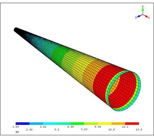
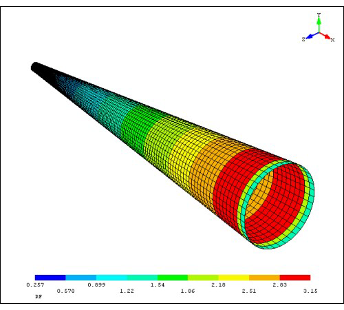
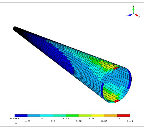
The analysis gives reserve factors (RF) as outputs.
The part resists load if
|---|---|---|
|FEA outputs for [0, 45, 0]SO lay-up |||
| |
| |
| |
|
|Compression|Traction|Flexion|
As shown on the images, the output spectrum is quite limited. The software displays few isosurfaces, just giving an idea of where the parts fails. As expected, the region of the tip is the most sensitive to stress. The images are essentially the same for the different lay-ups.
| | RF close to the tip |||
| Lay-up | Compression | Traction | Flexion |
|---|---|---|---|
| [0, 45, 0]S | 1.31 | 0.325, 0.756, 1.19 | 0.0209, 1.58 |
| [45, 0, 45]S | 1.23 | 0.285, 0.569, 0.853 | 0.203, 1.44 |
| [0, 45, 0]SO | 1.03 | 0.257, 0.578, 0.899 | 0.0166, 1.28 |
| [45, 0, 45]SO | 1.05 | 0.259, 0.512, 0.765 | 0.0172, 1.23 |
| [0, 45]S | 0.771 | 0.191, 0.413, 0.634 | 0.0124, 0.978 |
There is a very low risk of failing in the case of compression. All the values are above 1 for lay-ups with at least 5 plies. Even if the the results are not mesh independent, it can be seen on the image that apart from the very end tip, the other isosurfaces are well above 1.
- 2024_C_SE_ST_REQ_31ST Load Case - Axial compression

In the case of traction, the isosurfaces are identicals, in terms of localisation, compared to the compression case. However, there is a big region that is expected to fail. RF is above 1 only from the fourth isosurface to the last. The lay-ups are not rejected as most of the part resists to the load. Moreover, the requirement is not necessary appropriate. In real case, the nosecone will sustain a load far lower than the rest of the rocket during parachute deployment.
- 2024_C_SE_ST_REQ_33 ST Load Case - Axial deceleration

Failing regions are much more important in the bending case. They span up to the middle of the nosecone. However, similarly to the traction case, the requirement is far too severe compared to the real case. The bending moment applied corresponds to the maximum moment induced by the flight path correction by the fins. Therefore, the lay-ups are not rejected.
- 2024_C_SE_ST_REQ_34 ST Load Case - Bending moments

¶ Definitive lay-up
In short, the most pressing constraint is bending.
First of all, the lay-up [0, 45]S is rejected. It is the weakest lay-up among the list. It does not meet any of the load requirements.
Then, there are two types of lay-up: [0, 45, 0]x and [45, 0, 45]x (with x = S, SO). The FEA states that [0, 45, 0]x are better in terms of compression and bending. Moreover, in flexion, this lay-up type fails in compression whereas [45, 0, 45]x fails in shear in the principal directions. It is therefore, a safer choice to use [0, 45, 0]x.
As the analysis made is just for a preliminary sizing, the option with 5 plys is chosen to reduce mass and cost. Further analysis will be made to validate the choice.
Lay-up: [0, 45, 0]SO
Thickness = [mm]
[GPa]
¶ Bonding length
The nosecone is connected to the RE-Bay with couplers. This system is composed of a male part fitted into a female part which are glued to both bays. The connection is made by screwing the coupler together.
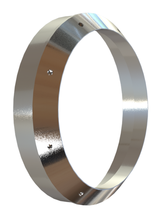
Due to the cylindrical geometry of a coupler, the nosecone must also incorporate a cylindrical surface.
The optimum bonding length is computed using a Volkersen model and Goland & Reissner model through an in-house Python code.
The parts to be glued together are inherently different. One is made of CFRP and the other one is made of aluminum. A toughened epoxy is used to glue them together, following the team's recommendation.
Also known as the shear-lag model, it introduces the concept of differential shear. In other words, it considers an asymmetric shear distribution in the lap-joint. This is mainly due to a difference in thickness between the two adherends.
The adhesive shear stress distribution is given by:
where,
- : characteristic shear-lag distance [mm] (i.e. a measure of how quickly the load is transferred from one adherend to other)
- : top adherend thickness [mm]
- : bottom adherend thickness [mm]
- : adhesive thickness [mm]
- : bonded area width [mm]
- : bonded area length [mm]
- : adherend modulus [MPa]
- : adhesive shear modulus [MPa]
- : force applied to the inner adherend [N]
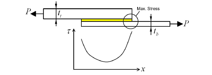
Principal of maximum stress for joints with different adherends
According to this model, there should be a concentration of stress at the interface between the thick adherend's root and the thin adherend. So, this zone is the first point of failure. Moreover, this assymmetry implies that is convex. In other words, the is maximised at an optimal length that gives . If the bonding length is significantly high, the adhesive cannot bear the deformation of the adherends, causing a failure.
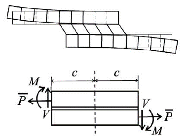
It considers the effects due to rotation of the adherends when a tensile load is applied (based on the finite deflection theory of cylindrically bent plates).
The adhesive shear stress distribution is given by:
where,
- : applied load per unit width [N.mm-1]
- : half of overlap length [mm]
- : adherend thickness [mm]
- : Poisson's ratio
- : bending moment factor
In contrast to the previous model, this one assumes that is a monotonic increasing function, which means that the greater the length of the bond, the better.
Adhesive: 3M Scotch-Weld™ EPX™ Adhesive DP490
Shear strength = [MPa] at 23°C & [MPa] at 120°C
On one hand, the Volkersen model does not consider two adherends made of different material. Hence, the modulus is assumed to follow a parallel law of mixing:
On the other hand, the Goland & Reissner model does not take into account a difference in thickness between the two adherends. The mean thickness is then, considered:
Assembly geometry
- [mm]
- [mm]
- [mm]
- [mm]
Material propertieshttps://www.matweb.com/search/DataSheet.aspx?MatGUID=c1ec1ad603c74f628578663aaf44f261&ckck=1
- [MPa]
- [MPa]
- [MPa]
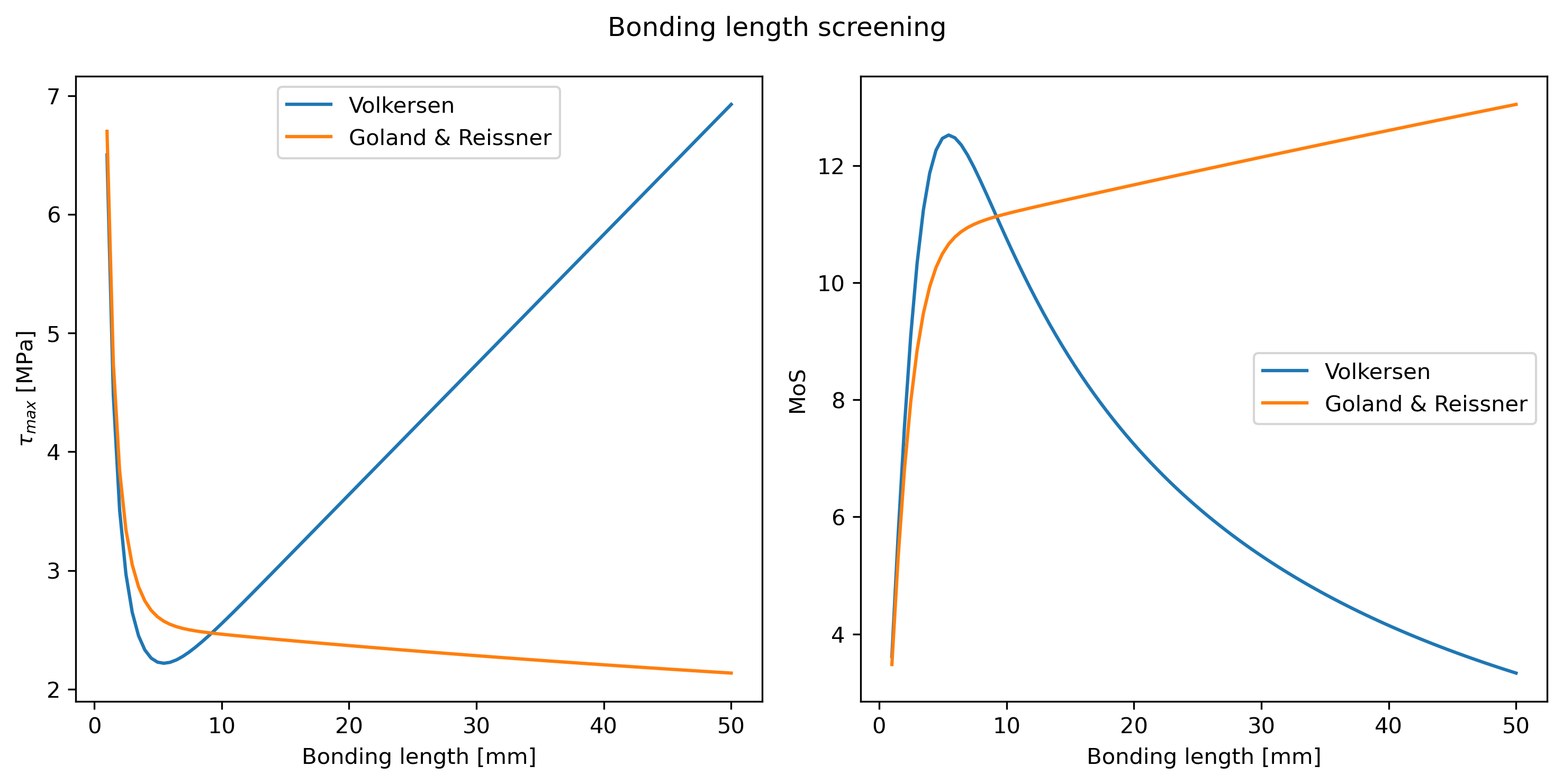
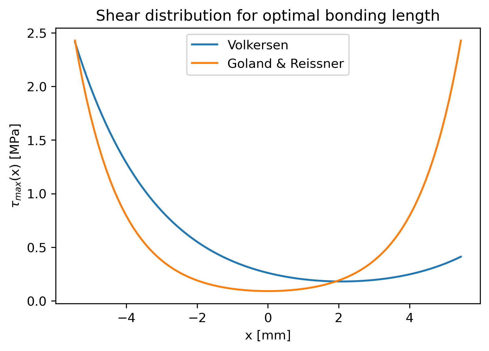
The optimal bonding length is given by the intersection of for the two models. This way, the length is not too high, preventing a premature failure at the interface of the adherends and, is not too low, avoiding a failure due to bending moment for low stress.
| Model | Length [mm] | Max shear [MPa] | MoS |
|---|---|---|---|
| Volkersen | 10.89899 | 2.414533 | 11.424761 |
| Goland & Reissner | 10.89899 | 2.428898 | 11.351283 |
Bonding length = [mm]
The is computed using the adhesive shear strength at 23°C. The worst case scenario would be a heating of the inner surface of the nosecone, causing a softening of the glue, giving a at 120°C. However, the nosecone shall be designed to resist to heat transfer, never allowing the inner part to reach such a high temperature during the flight.
For practical reasons, the cylindrical length is way bigger. It is hard to guarantee the coupling of the nosecone for such a low length. It is more convenient to assemble a coupler with a relatively large cylindrical length, especially for the concentricity. Moreover, having a longer coupler reduces the possible issues with non-parallel forces that might occur during the flight.
Cylindrical length = [mm]
¶ FEA
 2024_C_ST_NOSECONE-BAY_FEA
¶ Heat shield design
¶ Stagnation temperature
Stagnation temperature, also known as total temperature, is a thermodynamic concept used in fluid dynamics, particularly in aerodynamics and compressible flow analysis. It refers to the temperature of a fluid when it is brought to rest, typically by adiabatic compression. In simpler terms, if a fluid's motion were to suddenly stop, and it came to a complete standstill without any heat exchange with the surroundings, the temperature it would reach is called the stagnation temperature.
Stagnation temperature formula:
- : ambient temperature
- : air adiabatic coefficient
- : Mach number
The nosecone is designed to be able to withstand the stagnation temperature calculated at maximum speed. This conservative approach allows to anticipate for the worst-case scenario. In real case, the heat transfer is in transient regime, meaning that the airframe should not heat up to the stagnation temperature.
Atmospheric temperature model (https://www.grc.nasa.gov/www/k-12/airplane/atmosmet.html):
- : altitude ( [m])
- : temperature at sea level
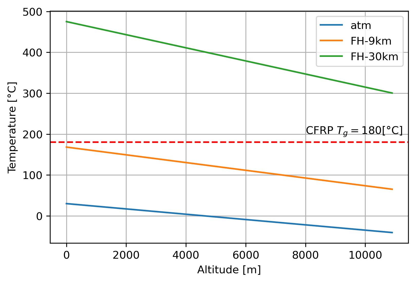
FH-9km and FH-30km fly respectively at [Ma] and [Ma]. In the model, [°C].
Flight at [km]: no need for a thermal protection
Flight at [km]: might need a heat shield
¶ Material selection
Heat equation:
In order to maximise the heating time, materials with low thermal diffusivity should be considered.
- : thermal conductivity [W.(m.K)-1]
- : density [kg.m-3]
- : heat capacity [J.(kg.K)-1]
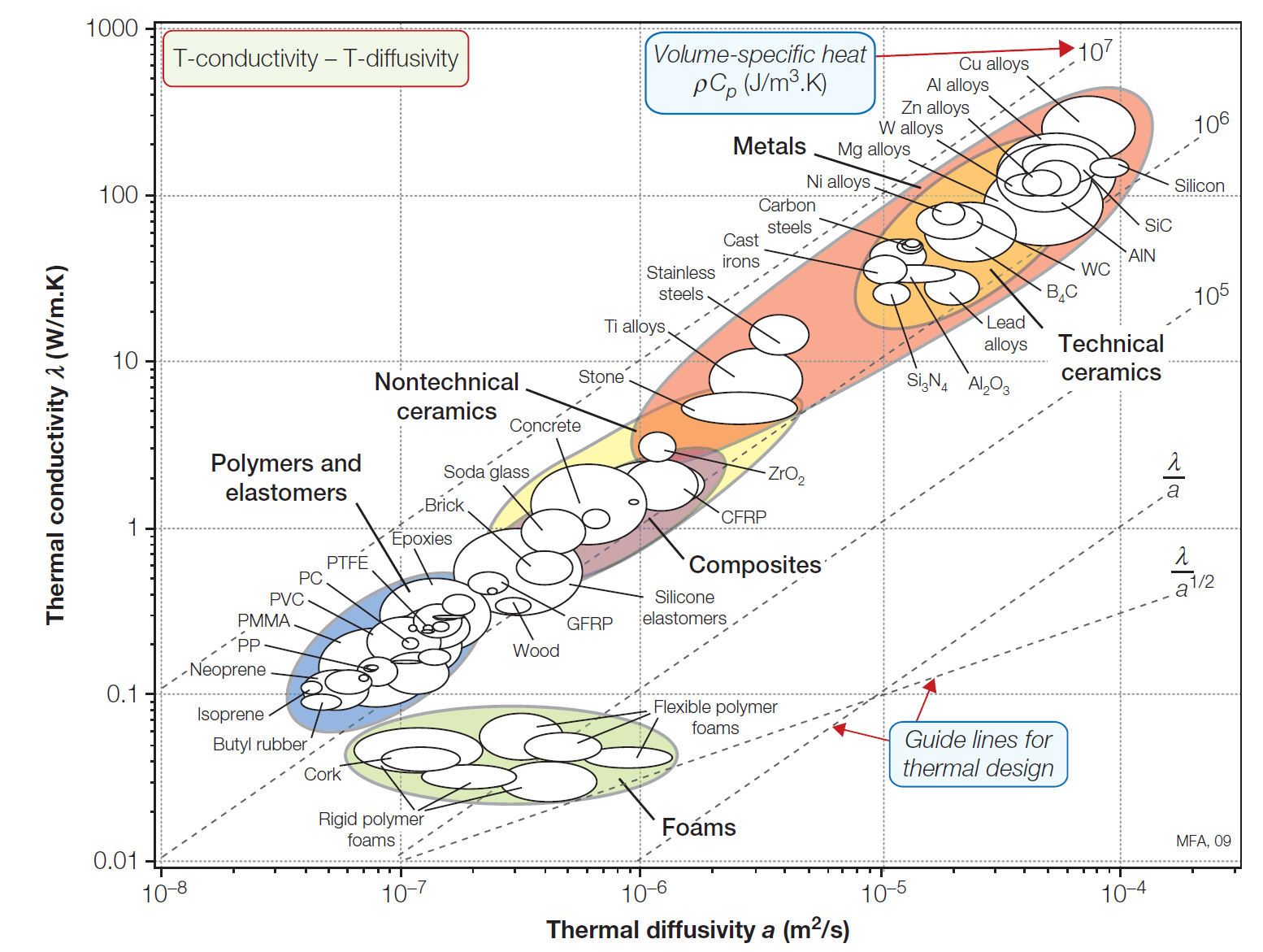
Polymers, elastomers and foams are good candidates for thermal protection in transient regime
The heat shield has to be either wrapped around the nosecone or us.ed as a coating. There is an additional constraint: the supply. The team should be able to afford and to buy it from an accessible supplier. In the previous year, the team worked with silica aerogel paint but without quantifying its benefits. Therefore, some analysis were performed to assess whether it can be useful or not. It is worthnoting that some research works were already made for more advanced thermal protection.
Additionally, radiation heating can also be a problem as the nosecone can stay under the sun for a long time when the vehicle is mounted on the launch pad. A metallic cover like survival blanket can be used for to mitigate this issue.
¶ Required thickness (steady state)
The heat shield shall stay in a transient regime while the engine is still burning (i.e. acceleration phase). This way, the outer surface of the nosecone should not heat during the ascent.
A simple numerical approximation of the 1D-Fourier's law is used to compute the time to reach a steady state. This approach assumes the heat transfer is diffusive and heat flows along a line. In fact, the curvature of the nosecone can be ignored as its thickness is very thin in comparison to its diameter.
Parabolic 1D problem
Space discretisation
Let and with . Let the approximation of at point . Using for the problem becomes:
In matrix form, the previous equation can be written as:
where, and a -matrix:
Time discretisation
A progressive Euler's scheme can be used to solve for time. Let the time step, with and, the approximation of at time . Using , the problem becomes:
Stability condition: \tau \leq \frac{h^2}
Heat shield
- Material: Gore® Silica aerogel coating
- [W.(m.K)-1]
- [kg.m-3] (adhesive + aerogel)
- [J.(kg.K)-1]
- [mm]
Boundary conditions
- for
Numerical parameters
- [mm]
- [s]
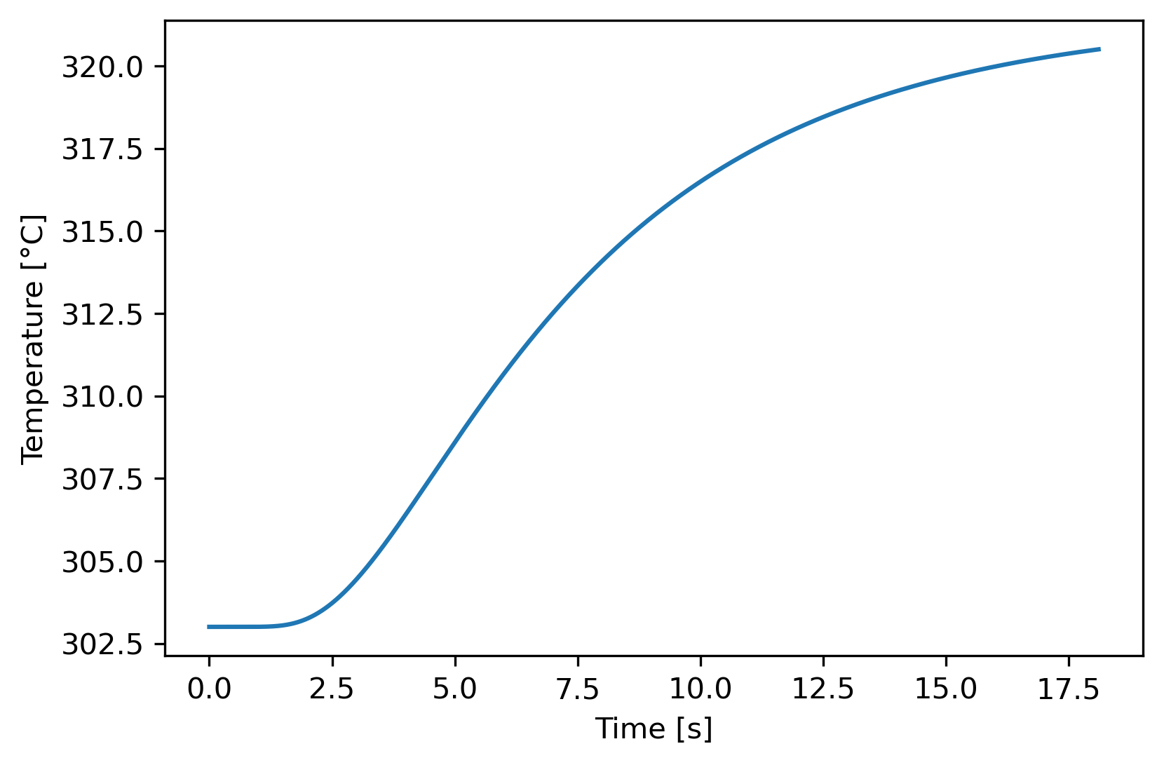
Transient heating at point
A Python code is ran until [K]. When this condition is satisfied, it is assumed that the diffusion as reached a steady-state
The transient regime lasts for: [s] [s], the burn time
It is worth noting that a heat shield might be unecessary as the model is considering an unrealistic boundary condition on the skin. First, the vehicle will stay at its maximum speed for a very short time ( [s]). Then, it will reach that speed at high altitude, meaning that the ambient temperature is low. The airframe will hence start to cool down quickly. Lastly, some thermal resistance tests have been conducted on a similar carbon: HexPly® 8552/40%/160WUD/AS4C-3K (3.8[mm]). It has been reported that the epoxy matrix starts to decompose at 511°C with a heating speed of 1000 [°C/min] and under a compressive load of 100 [N]. This finding suggests that as long as the nosecone does not reach and stay at ~500°C for a long time, it will not degrade because of thermal stress.
¶ Perspectives
- Tip
It has been reported that manufacturing a CFRP tip with prepregs laying-up can be difficult as all the overlaps from plies will stack on the tip. A solution can be machining a tip in aluminium or 3D-printing a high temperature resin instead of laying-up a CFRP tip. The CFRP nosecone will then be truncated for the manufacturing. - Heat shield
FEA will be needed to refine the material selection as well as the coating thickness. Therefore, FD division have to provide the appropriate temperature field.
¶ Relevant Documents
- “Nose Cone Design.” Wikipedia, 22 Jan. 2024. Wikipedia, https://en.wikipedia.org/w/index.php?title=Nose_cone_design&oldid=1198011130
- ST - Thermal protection systems of a spaceshot rocketStudent: Vincent Ben-Thlija
Supervisor: Prof. Veronique Michaud, Alexandre Looten - ST - Delamination of carbon fibres during a spaceshot flight Student: Noah Studer
Supervisor: Prof. Veronique Michaud, Alexandre Looten