¶ title: Antennas
description: Doc ID: 2023_ANTENNAS_TN_B01
published: true
date: 2025-05-21T19:03:17.852Z
tags:
editor: markdown
dateCreated: 2023-07-19T11:07:06.103Z
¶ title: Antennas
description: Doc ID: 2023_ANTENNAS_TN_B01
published: true
date: 2024-12-30T21:15:52.790Z
tags:
editor: markdown
dateCreated: 2023-07-19T11:07:06.103Z
¶ title: Antennas
description: Doc ID: 2023_ANTENNAS_TN_B01
published: true
date: 2024-01-29T23:25:54.178Z
tags:
editor: markdown
dateCreated: 2023-07-19T11:07:06.103Z
¶ title: Antennas
description: Doc ID: 2023_ANTENNAS_TN_B01
published: true
date: 2023-07-19T11:07:06.103Z
tags:
editor: markdown
dateCreated: 2023-07-19T11:07:06.103Z
¶ AV Antennas
¶ 1. Introduction
Demonstrated Wizardry: the wireless telegraph is not difficult to understand. The ordinary telegraph is like a very long cat. You pull the tail in New York, and it meows in Los Angeles. The wireless is the same, only without the cat.
The aim of this Technical Note is to give technical information about the antennas themself, as well as providing useful information to the team on the different considerations that need to be accounted for when designing a wireless system that involves antennas.
¶ 2. Reference Documents
| Ref | Description | Doc. ID | Issue |
|---|---|---|---|
| [RD01] | Antenna Technical Note | 2022_AV_TN_B09 | R01 |
¶ 3. Definitions and Abbreviations
- AV: Avionics
- FD: Flight Dynamics
- GS: Ground Segment
- GST: Ground Station
- PL: Payload
- PR: Propulsion
- RE: Recovery
- SE: Systems Engineering
- ST: Structure
- HPBW: Half Power Beamwidth
- LHCP: Left-Handed Circular Polarisation
- LP: Linear Polarisation
- LV: Launch Vehicle
- MAG: Microwave and Antenna Group
- RSSI: Received Signal Strength Indication
- VNA: Vector Network Analyzer
- EE: Electrical Engineering
¶ 4. Antenna theory
¶ 4.1 The concept of antenna
From an electrical point of view, it is in charge of transforming a planar electromagnetic wave, the input signal, to a spherical electromagnetic wave. Thus, an antenna obeys the Maxwell equations.
One should be careful when applying known EE basic concepts such as voltage or currents, as they sometimes result from approximations only valid at low frequencies, which is definitely not the case in antennas. The antenna is a device that does not follow Kirchhoff's laws, and that can not be modelled as a dimensionless object, or a point object. Transmission lines model, waveguide models and Maxwell equations are more suitable in these cases, because it really implies wave propagation.
¶ 4.2 Propagation and signal decay
As mentioned previously, the antenna propagates a signal through a spherical wave. This means that as the receptor moves away from the source, the power at the receiver diminishes, simply because of spherical propagation. This phenomenon is often referred to as path losses, and will also be called that way in this document. This does not include any dissipative losses. This path losses are proportional to the square of the distance, and the square of the frequency.
This signal decay is what limits the range of operation of the system, and is therefore a major constraint. This will be accounted for in the calculation of what is called a link budget. This establishes the ability of the system to communicate over a certain range, or to determine the maximum operating distance.
¶ 4.3 Antenna radiating principle
The simplest case of radiating antenna is the electrically small dipole. The electric field is maximum at both extremities, but with an opposite sign, which makes the electric field around to be curved, and then propagates in spherical waves, far enough from the antenna.
All antennas are working following a similar principle, and engineering them allows optimising different trade-offs for different applications, such as gain pattern, bandwidth, polarisation, etc.
¶ 4.4 Polarisation
Each antenna has a certain type of polarisation. The polarisation mismatch of the antenna is a source of losses. Intuitively, it can be seen as the misalignment of the electric field produced by the transmitting antenna and the one that the second antenna can receive. In the best case, it results in a 0 dB loss, and in the worst case it can be , completely blocking the transmission.
Formally, the depolarisation factor can be calculated as:
And in term of power:
Where are the polarisation vectors of the receiving antenna, respectively the transmitting antenna. The design choice this year is to make the GS antenna circularly polarised, and the rocket's antenna linearly polarised. This results in a controlled permanent loss of regardless of the orientation of the rocket.
¶ 4.5 Link budget
First step is to establish the link budget (all quantities in dB, dBi or dBmW):
Where:
- is the received power, which should be above the receiver sensitivity.
- is the transmitted power
- the gain of the transmitting antenna
- the gain of the receiving antenna
- the path losses, being the distance of the transmission, the operating frequency
- the losses due to polarisation mismatch
- the losses due to pointing mismatch
- due to diverse mismatches (cables, reflections, etc)
Note that the received power is the power received at the receiver, and the receiver sensitivity is the minimum power required at receiver to work, mostly dependent on the noise of the receiver electronics.
This ensures that communication is possible, or what is the maximum range of operation. Note that the path losses can be higher due to reflection in an urban environment. In this case, since the communication with the rocket is almost direct, these effects are not relevant.
Dispersive effects are not included either, because they are not dominant and can depend on unpredictable parameters such as weather. Ultimately, they will also impact the communication range.
The link budget is therefore a rough estimation of the constraints on the systems, which aims at providing initial guidelines for a design. One should keep enough margin for degraded performance due to secondary effects.
¶ 5. Main antennas
¶ 5.1 Link Budget
The link budget is established, with the following parameters:
It leads to a margin of 0 dB in the link budget. However, since the margin taken in account in the is already a pessimist estimation, there is no need to take additional margin. It means for the design of the antenna that its minimal gain should be greater than -5 dB.
¶ 5.2 Design flow
The design is investigated through a simulation software: HFSS from Ansys. One should be very careful with the convergence of the simulation, and learning intuition on how to set simulation parameters to have trustworthy results is very useful. The software adds iterative mesh elements until consecutive passes are similar enough. The key parameter for similarity between two passes is the parameter. We have chosen to set this value to 0.01. The number of maximum passes can also be chosen to avoid losing too much time when only rough results are needed. With the increasing complexity (adding lossy materials, complex geometry, etc) of the antenna model, the number of passes to achieve convergence increases.
It is necessary to have a good design procedure to avoid losing time in simulation, as it is easy to be overwhelmed by the number of parameters to tune in the antenna. In order to do so, it is good to get an intuition of how basic parameters influence the main characteristic of the antenna, and to which extent they do it. The design flow is an iterative process, beginning from a simple antenna, in free-space, without the rocket, on a flat substrate. Later, more complexity will be added to the model in order to get closer to the physical reality.
¶ 5.2.1 Constraints
The body of the rocket is made out of carbon fibre, which is electrically conductive. Thus, it acts like a shield for electromagnetic waves, and does not allow communication through. Therefore, the antennas are placed outside the rocket, and should be as thin as possible. The carbon fibre will act as a ground plane, and as a consequence, the antenna should be as far as possible from the body to avoid destructive interference (see electromagnetic image theory for more details). One way to mitigate this phenomenon while still keeping the antenna close to the rocket is to choose a substrate with the highest largest dielectric constant . The substrate should be bendable, and ideally low-losses to maximise the efficiency of the antenna. Some tests done the previous years showed that RT/duroid® 5870 Laminate is sufficiently bendable and has the required electrical properties.
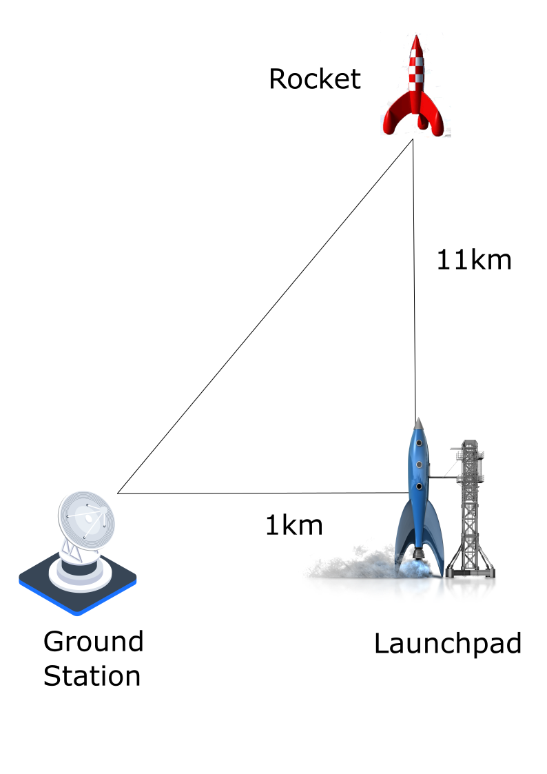
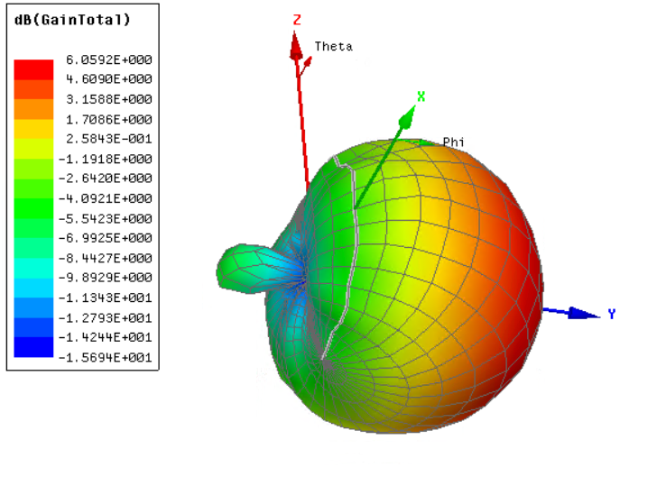
Another constraint is a geometrical one. As the rocket is at its apogee, it is 10 km away from the GST, at an angle of which is very different from the rocket at the launchpad, where the angle is . This means that the antenna gain should be sufficient along to . The worst case is at , which will be used as a design constraint.
¶ 5.2.2 Antenna typology
The chosen antenna is a square patch because of its suitable gain pattern and its simplicity. The antenna on the rocket is LP, while the ground station one is LHCP. This ensures that we have a constant loss of 3 dB due to polarisation mismatch, regardless of the orientation of the rocket.
To first get an initial sizing, online calculators are sufficient, and it avoids losing too much time in the simulation. The one used here is https://www.everythingrf.com/rf-calculators/microstrip-patch-antenna-calculator and gives a rough estimation of a square patch of 130 mm. However, understanding the functioning of the antenna is required to know which metric needs to be modified.
First, the calculator suggests having different dimensions for the length and the width, which would make a rectangular patch. However, it is not desirable because there is a risk of exciting multiple modes and the feeding point would be harder to choose. The chosen structure is thus kept as a square patch.
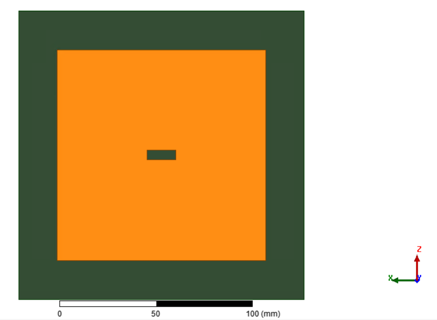
¶ 5.2.2.1 Miniaturisation
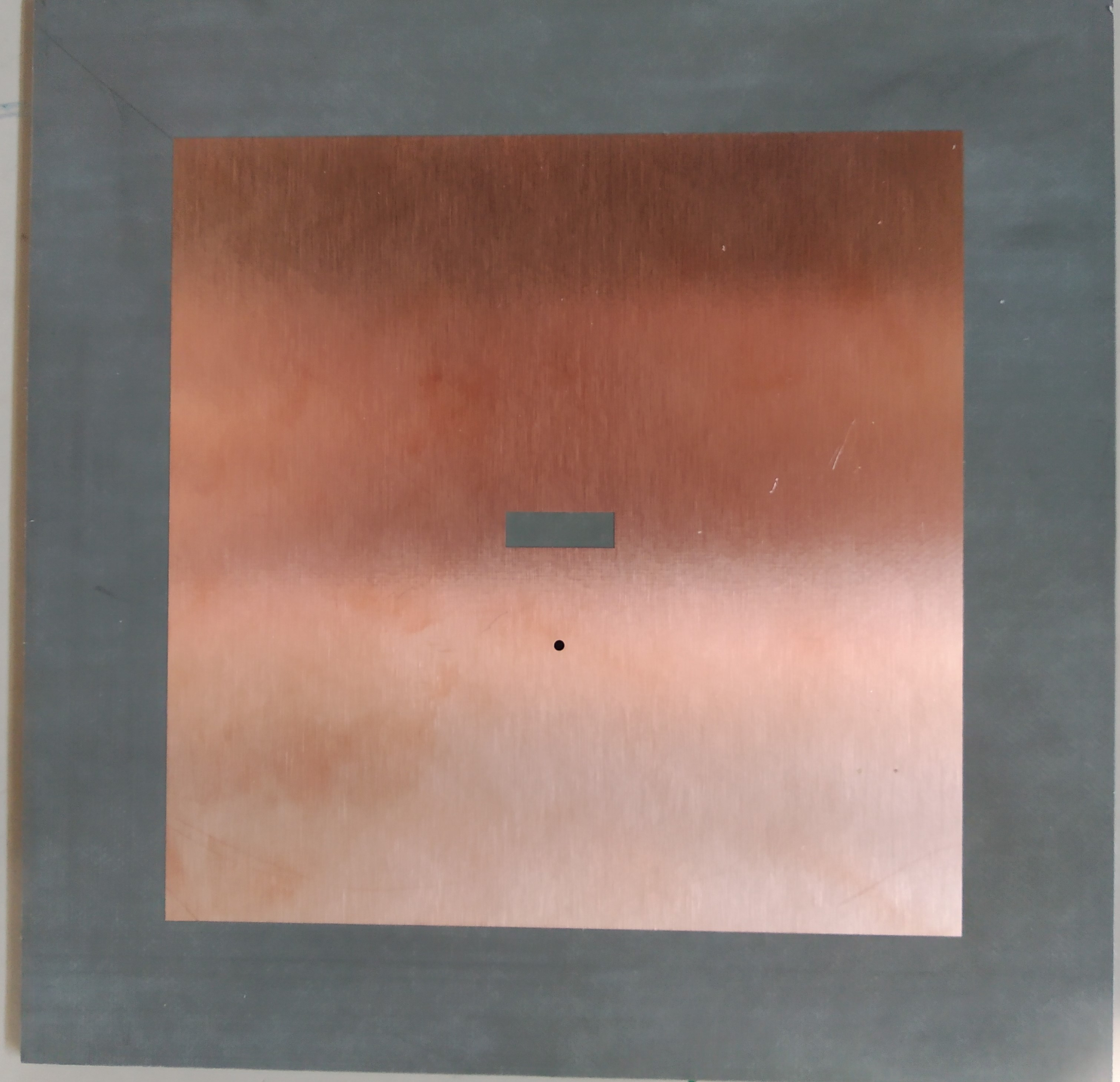
The physical constraints, mainly the circumference of the rocket, do not allow for a simple patch design which would be too large. Therefore, the final design is slightly different and requires miniaturisation techniques. We explored two of them: one is short cutting the antenna at the middle along the Z axis,and the other is cutting a rectangle aperture at the centre of the antenna. The first principle works as in the excitation of the mode the electrical field is zero along the Z axis. Short cutting the antenna at this position allows it to keep the same boundary conditions, and therefore the same radiation while getting rid of half of the antenna. However, due to the very thin thickness of the substrate, the tuning process was too sensitive, and the risk of having the antenna not working after the production phase was too high. We therefore explored the other miniaturisation technique: the slotted patch. It artificially increases the electrical length of the antenna because the currents lines along the Z axis are slightly longer, therefore decreasing the operating frequency while keeping the antenna small enough.
The parameters to tune are then: the length of the slot, its width, the width of the antenna itself, and the location of the feeding point. To avoid exiting other modes, the feeding point is kept along the Z axis, which means that only its Z coordinate can be moved.
The width of the antenna is the main parameter that defines the resonant frequency of the antenna. The larger it is, the smaller the operating frequency. Enlarging the size of the slot allows to decrease the resonant frequency, while keeping the width constant, at the cost of a lower efficiency. Therefore, the width is set to the maximum allowed by physical constraints, and the size of the slot is used to finetune the resonance.
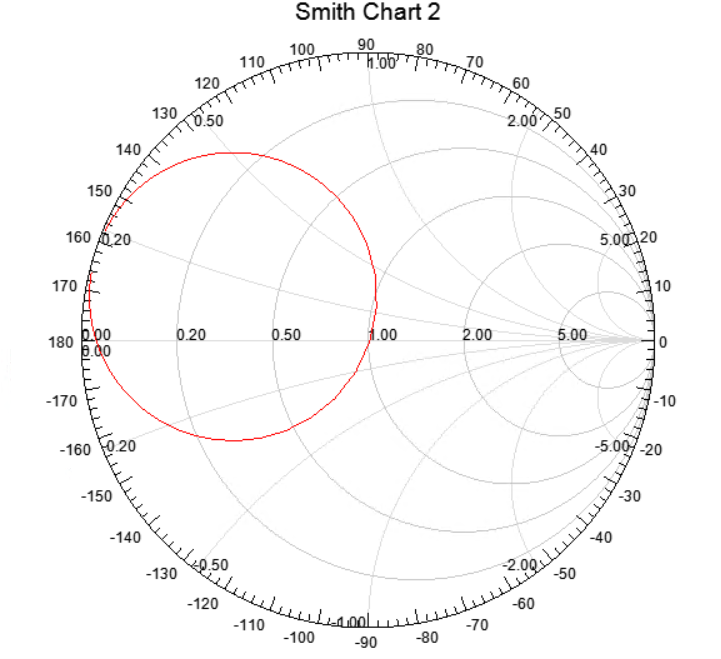
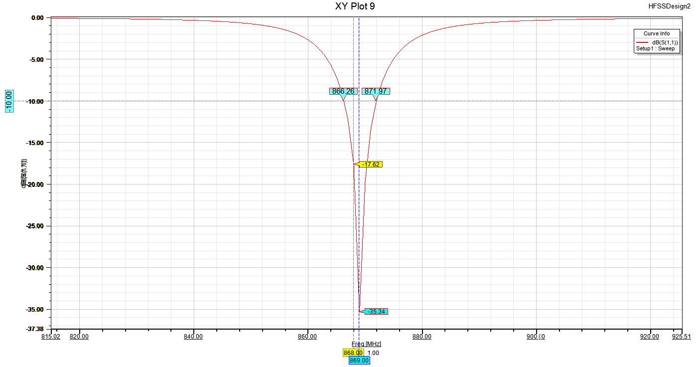
¶ 5.2.2.2 Impedance Matching
Another very important point is the matching of the antenna. To maximise the power transfer from the amplifier to the antenna, it should be matched. This means that the impedance of the antenna is the complex conjugate of the port:
The reflection coefficient is then defined as
As it is often the case, the previous stage has an impedance of 50 and the antenna is then matched to this impedance. This is done by moving the feeding point on the Z axis. The ratio of electric field and magnetic field at a given point sets the impedance, and since the electrical field is at its maximum at extremities, and almost zero along the X axis at z=0, the impedance is small close to the slot, and increases as the feeding point is moved away, closer to the edge.
The reflection coefficient can be observed in magnitude on the right plot of Fig. 2 or on the smith chart, on the left of Fig.2. The should be minimal at the operating frequency, and low enough around to allow a sufficient bandwidth. As it can be seen, simulations show that the antenna are matched to 869MHz with a but can still be used at 868MHz at the cost of a worst matching: . The bandwith is then 6MHz, largely sufficient for the LoRa requirements.
Once a good matching is achieved and the antenna has a sufficiently high radiation efficiency, it can be sent to production.
¶ 6. GPS antenna
- f = 1.5 Ghz
- Square patch of 100 mm x 100 mm
¶ 6.1 Design flow
¶ 6.1.1 Constraints
Since the operating frequency is higher, the patches are smaller and do not need to be miniaturised. Thus its design is simpler, and a more basic typology will be used than for the main antennas.
¶ 6.1.2 Antenna typology
A simple square patch is adapted to the right frequency, and matched to .
¶ 6.1.3 Testing
Since the design methodology has already been confirmed with the main antenna, the only test done here is the reflection coefficient, measured on the VNA.
¶ 7. Wifi antennas
- f = 2.45 Ghz
- Square patch of 60 mm x 60 mm
¶ 7.1 Link Budget
The link budget is established, with the following parameters:
This leads to a margin of 5.95 dBm. Note that the power transmitted is this high because of the use of an amplifier.
¶ 7.2 Design flow
The design flow is identical to the one of the main antenna, except that the constraints are changed a bit.
¶ 7.2.1 Constraints
The major difference is that due to its high frequency of operation, the antenna will be much smaller. This means that it is very unlikely that the antenna requires miniaturisation, thus the design process will be simpler.
¶ 7.2.2 Antenna typology
The antenna is a square patch, on a ground plane. Its length is tuned to resonate at 2.45 GHz and the feeding point is placed such that only one mode is exited and the antenna is matched to .
¶ 7.2.3 Testing
Since the design methodology has already been confirmed with the main antenna, the only test done here is the reflection coefficient, measured on the VNA
¶ 8. Conclusion
Designing an antenna is not as complicated as it seems, but one should pay attention to the fundamental concepts of electromagnetic propagation. A part no to underestimate is the mechanical part during the fabrication. Getting help and advices form the structure team was welcome and helpful.
¶ 9. Acknowledgements
We want to thanks Rogers Corporation that kindly provided RT/duroid® 5870 Laminate samples for the substrate.
We also want to thank the MAG at EPFL for providing the infrastructure, the test facility as well as the precious advice.