¶ Goal(s) of the study
This study is a continuation of the Pressurant Bay Dynamical Analysis 2025_C_ST_PBAY_DYNFEA. The Pressurant Bay Dynamical Analysis served as more of a "training ground" for these analyses, and as such, this report more complete, studies and compares more cases, and is generally more of a corner stone to this Bachelor's Project.
Here, we are looking to characterize the dynamical effects of the motor and fins on the Engine Bay instead of the Pressurant Bay, as done before.
This analysis looks to expand on the previous work by completing multiple analyses to expand on the previous ones: different time steps and analysis settings allow us to have a closer look at transient effects, while still studying steady state results.
In this analysis, we will also be using 3 different ABRs, which allow us to tie this analysis to the Bachelor Project see if composite ABRs provide a noticeable different in dynamic situations (they have only been studied statically for buckling uptil now).
¶ Parts Involved
¶ Geometry
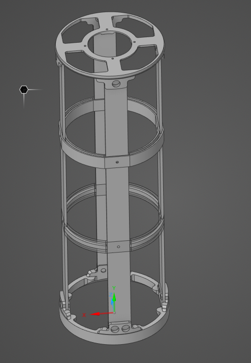
The Geometry used is the Engine Bay assembly, composed of the coupler, thrust plate, rods, and ABRs.
All screws were removed to simplify the analyis, alongside the rail button and fins attachments.
4 CRFP Rods
2 Aluminum ABRs
1 Coupler
1 Thrust Plate
¶ Function
The Engine Bay is the launch vehicle's engine housing module. The B1 is placed on the thrust plate, such that all thrust is transmitted through this part to the rest of the internal structure. The rest of the engine bay's space houses the plumbing required to run the liquid oxygen and ethanol to the motor, as well as housing the igniter.
The internal structure, of course, ensures the rocket's structural integrity, supporting the engine's thrust (compression load), the lateral acceleration caused by the fins, and the parachute's tension loads.
¶ Material
The different parts of the assembly are made of different materials
- Rods: these rods are made of CFRP, who's layup is described here: 2024_C_ST_CFRP-PLATE_MAP
- Couplers: the couplers are made of Al2050-T84
- Thrust Plate: the thrust plate is made of Al2050-T84
- ABRs: the ABRs are made of either Al2050-T84, or CRFP and PETCF spacers, depending on which analysis
Material properties are descrived in more depth later on in the document
¶ Load case
The loads applied to the pressurany bay are, most notably:
- Motor Thrust: Compressive Forces (7.5kN for FH1, 15kN for FH2)
- Parachute Opening: Tension Forces
- Fins Force (Lateral Acceleration)
In this analysis, we focus on the motor and fin forces, in the first 10 seconds of flight.
We will be studying 3 different load cases, which will be explained later on in the FEA section of the report, but for all the load cases, we got the forces as follows:
¶ Fins
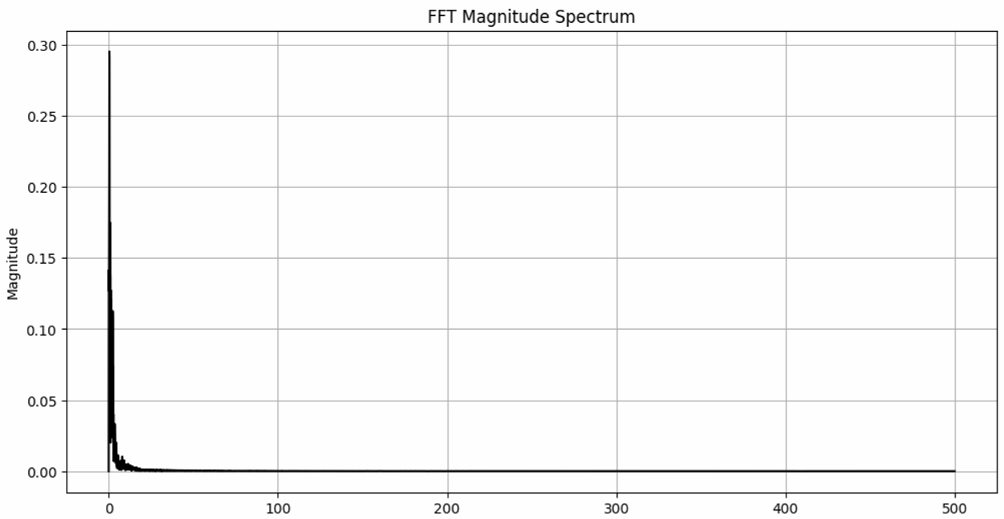
The fins lateral acceleration was found using the Open Rocket simulations for Firehorn 1, at full thrust on 7.5kN. Once the lateral acceleration was obtained, a Fast Fourier Transform was done on this data, from which the 10 most dominant frequencies were used to reconstruct the acceleration, followed by the force (F = m * a with m = [x] kg). These corresponding graphs are shown here:
¶ FFT Magnitude Spectrum
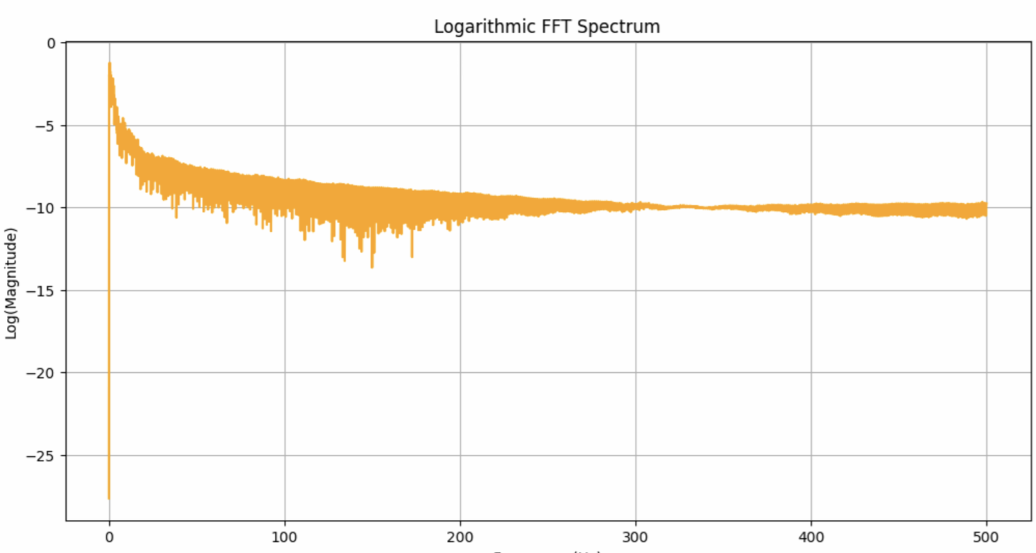
¶ Logarithmic FFT Magnitude Spectrum
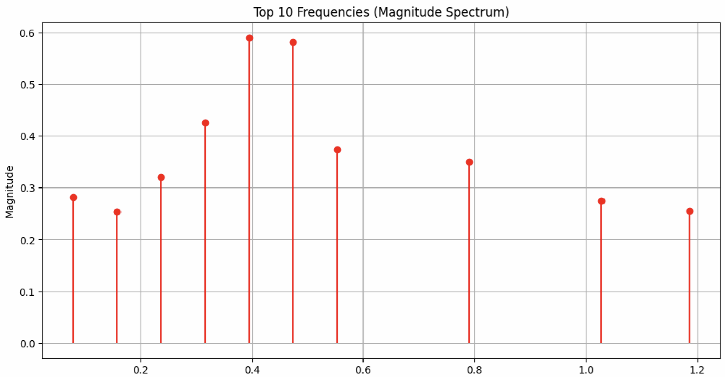
¶ Top 10 Frequencies
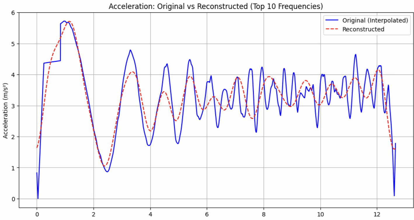
¶ Reconstructed Acceleration
¶ Reconstructed Force
.png)
¶ Motor Thrust
Motor thrust is taken from the expected thrust as the motors are designed: 15kN for the C engine. The thrust curve itself is taken from the Rocket Team's Testing Facility's experimental results (done on the B engine, but shouldn't be too dissimilar).
The choice was made to take the 15kN force of the C engine even though it is only on the FH2 vehicle (while the fins forces are those of the FH1 vehicle) because on the Pressurant Bay analysis, the fins' force was neglible compared to the 7.5kN force.
We keep the fins force in the simulation as they provide more information without adding too much computational load, without falsifying the results. If time allows, a 7.5kN simulation with the fins forces will be added to the results.
¶ Parts List
¶ Finite Element Analysis
¶ Software
- ANSYS Mechanical (2024 R2)
¶ Type of simulation
A transient structural simulation is performed. To make this simulation computationally less time consuming, we use the Mode Superposition (MSUP) method. This means we perform a modal analysis on the assembly first, and use this as an input to the transient structural analysis. As an example, one of the preparatory simulations took 12* more time without the MSUP method (90minutes against 7min).
ACP Pre was used for the composite ABRs, the set up being explained in the "Inputs" section.
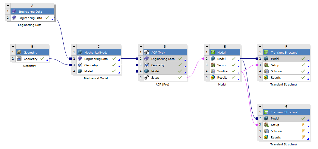
This setup looked as follows, with additional blocks being used to run different simulation set ups with the same assembly/material data.
Important: when connecting ACP Pre to Modal Analysis (or Static Structural, or Transient Structural) you must drag the "Setup" from the ACP Pre tab to the "Model" of the next tab, and click "Transfer Shell Composite Data" when using Shell, or Solid when using Solid. In all of this project's analyses, shell data was used for the simplicity it comes with.
¶ Inputs
The inputs will be split into 2 cases, where the units, geometry modelling and material modelling don't change case to case (except for ABR material) and the time modeling and boundary conditions change. These 2 cases will be reflected in the Outputs, as well as a final comparison section.
- m-kg-N-Nm-Pa-m^4-J
For this analysis, the geometry was quite significantly modified (compared to other ones in this project).
- The screws and nuts are removed
- Most of the screw holes are removed
- The screws' pilot holes on the rods <> coupler/rod <> thrust plate contacts were removed
- The rail button and fin attachments were removed
- All contacts are defined as "bonded"
The core geometry shapes were kept as is, but many of these small details (holes) were removed in the hopes of simplifying the mesh, thus improving mesh quality, decreasing quantity of nodes, and improving computation time.
¶ Thrust Plate, Coupler, and Aluminum ABRs:
- Aluminum alloy 2050 T84
{.links-list}
| Density (g/cm^3)| Young's Modulus (GPa) | Poisson's ratio |
|---|---|---|
| 2.7 | 76.5 | 0.33 |
¶ Rods
- CRFP (UD)
The CFRP properties have been defined using ACP.
The properties for the UD and woven plies are:
| Material | Density (g/cm^3) |
|---|---|
| UD | 1.47 |
| Woven | 1.49 |
|||||||||||
| | Elastic (Engineering constants) |||||||||
| Material | E1 | E2 | E3 | Nu12 | Nu13 | Nu23 | G12 | G13 | G23 |
|---|---|---|---|---|---|---|---|---|
| UD | 137000 | 10500 | 10500 | 0.3 | 0.3 | 0.51 | 5200 | 5200 | 3476.82 |
| Woven | 49000 | 49000 | 10000 | 0.05 | 0.35 | 0.35 | 5000 | 4500 | 4500 |
In ACP, the layup from 2024_C_ST_CFRP-PLATE_MAP was defined, which gave the following properties for the CFRP rods using an orthotropic model:
| Density (g/cm^3) | E1 | E2 | E3 | Nu12 | Nu13 | Nu23 | G12 | G13 | G23 |
|---|---|---|---|---|---|---|---|---|
| 1.5 | 88074 | 17739 | 10000 | 0.3 | 0.3 | 0.3 | 3500 | 4081.6 | 3192.2 |
To correctly apply the material for the rods, a coordinate system is defined for each rod, with the X, Y and Z axis oriented so that the properties are in the same direction as for the actual rods.
¶ Carbon Fiber ABRs
¶ PETCF
The DLL's PETCF's Datasheet provided the Young's Modulus as well as the density, from there, we found the Poisson Ratio based on research of other similar 3D printed materials (PETG) and we found the Shear Modulus using the formula to find G based on E and the Poisson Ratio.
|||||||||||
| | Elastic (Engineering constants) |||||||||
| Material | E1 | E2 | E3 | Nu12 | Nu13 | Nu23 | G12 | G13 | G23 | Density |
|---|---|---|---|---|---|---|---|---|---|
| UD | 6030 | 6030 | 3200 | 0.38 | 0.28 | 0.28 | 2185.5 | 2355.5 | 2355.5 |1.3g/cm^3|
¶ Carbon Fiber
The properties for the UD plies are:
|||||||||||
| | Elastic (Engineering constants) |||||||||
| Material | E1 | E2 | E3 | Nu12 | Nu13 | Nu23 | G12 | G13 | G23 | Density |
|---|---|---|---|---|---|---|---|---|---|
| UD | 130000 | 8600 | 8600 | 0.27 | 0.4 | 0.27 | 4700 | 3100 | 4700 |1.55g/cm^3|
The E1 and density were taken from the UD prepreg's datasheet - the rest was kept as standard values from Ansys' material libraries (which were compared to standard UD CRFP).
The ACP module was then used to set up the lay ups, so the values of the entire module are calculated by Ansys.
All cases are transient simulations
None of these cases are a perfect represenation of the case we are looking to simulate. The "perfect" case would be about 11s of motor burn, followed by ~10s without burn to simulate the transient effects.
A 10s simulation of our models with a 0.01s time step generates a 134Gb file.
Unfortunately, to capture transient effects, the required time step is 0.0001s (0.1ms) - this time step paired with a 10s simulation should generate a file of about ~13Tb.
Even the perfect case at a 0.01s time step of 20s would create a ~270Gb file.
This left us in front of a trade off:
- Simulate a 2x time scaled analysis with a 0.01s time step, but miss the transients. This timing is sufficient to reach a steady state in the analysis.
- Simulate a 20x (50ms) time scaled analysis with a 0.0001s time step, to capture transients, but without being sure it is a valid simulation.
The time steps were scaled even further down, as file sizes increased dramatically when using ACP Pre (initial calculations were done with the Aluminum ABRs). The timings were divided by two for both the full burn and the short scale, leading to 800Gb file sizes.
The timings simply reflect the application of the force, which are described in the boundary conditions, and the time step was chosen based on what we were looking for (the "steadier" state solution, or the transients: case 1 vs case 2).
The exact implementation was iterated on to find these final set ups.
¶ Case 1 "Full Burn"
This analysis looks to emulate a full motor burn. The timings simply reflect the application of the force, which is described in the boundary conditions
-
Time Step: 0.01s
-
Analysis Settings (Timing)
5 Steps - 5s duration
1st Step: 0.25s
2nd Step: 0.3s
3rd Step: 2.5s
4th Step: 2.55s
5th Step: 5s
¶ Case 2 "Short Scale"
This analysis looks to scale down the full motor burn, to capture transient effects, albeit imperfectly.
- Time Step: 0.0001s (0.1ms)
- Analysis Settings (Timing)
5 Steps - 50ms duration
1st Step: 0.0125s
2nd Step: 0.015s
3rd Step: 0.125s
4th Step: 0.1255s
5th Step: 0.25s
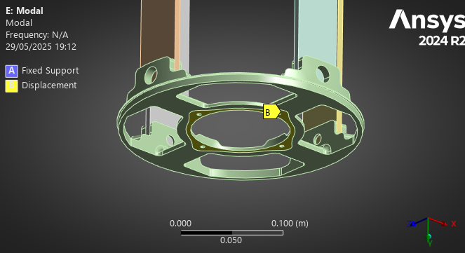
The thrust plate's X and Z displacements were set to 0, as the motor should only act in the Z direction, and to simplify the analysis.
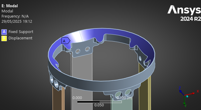
The coupler's movement was fixed, as it is "fixed" to the upper modules in flight.
A compressive (upwards) force of 15kN is applied to the thrust plate's motor fixation.
The fin's forces were initially applied as a moment to the top coupler, simplifying the reality of the force. However, using a "Remote Force" it was possible to apply the force at the location of the rocket's Center of Pressure (where aerodynamic forces are applied), while being applied to the couplers' sides.
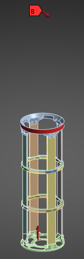
We had to simplify the direction because Openrocket only returns a magnitude for the lateral acceleration, not a vector - so this is somewhat of a "worst case" scenario). In any case, the deformation caused by the fins is so minimal it doesn't even appear relative to that cause by the motor.
The forces for Case 1 and Case 2 are identical, but "scaled down" in time for both.
¶ Both Cases
The force table for the motor looked like this:
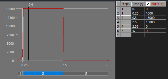
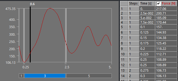
The force function for the fins looked like this:
| Real case | Model |
| Attached to another module | Fixed |
| Compressed due to lift off | Compression force |
| Lateral forces due to fins | One Direction Force Laterally to the Couplers |
The most important elements of the settings are:
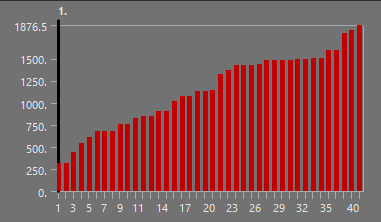
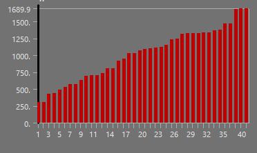
- Modal Analysis before Transient structural, where we found 40 modes. We used 40 modes because the 40th mode was at 1500Hz, which is the drop off point for the Forces' Frequencies (Laplace Transform on a Ramp/Step for the Motor, and FFT for the Fins).
- Damping Ratio set to 0.02 in Transient Structural
¶ Mesh
Quadratic Elements were used with the "Automatic" element type. The automatic element type allowed us to reach the highest quality, and Hex Dominants were not adapted to these models who's surface to volume ratio is too high - leading to meshing failures.
"Quality" was set to 0.95 in Ansys.
No refinements were applied.
Unfortunately, given the shear size of these simulations (upto 880Gb), the length of these simulations (upto 4 hours) and the time constraints of a due date for this project, executing an ideal mesh independency tests on the specific simulations done in this project was unrealistic - decreasing the mesh size lower than what we used would simply not have fit in our computers (for which 1Tb of storage was bought).
The choice of the mesh was the same as the ones used in the previous analyses: 2025_C_ST_COMPOSITE_ABRs_FEA, where a mesh independency test was performed on the first buckling mode. This is not ideal, but it should be sufficient. The similarities in results between the outputs of the aluminum and composite ABRs as well as the different time scales is somewhat reassuring in this regard.
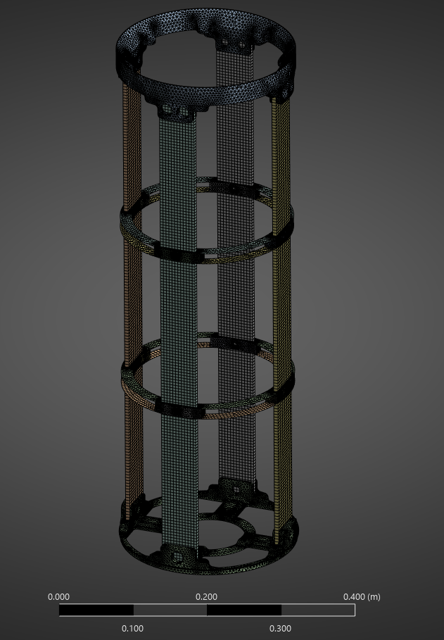
The final mesh between all ABRs was identical, 5mm for the rods, couplers, and thrust plate, 3mm for the ABR components.
Here is a complete view of the mesh:
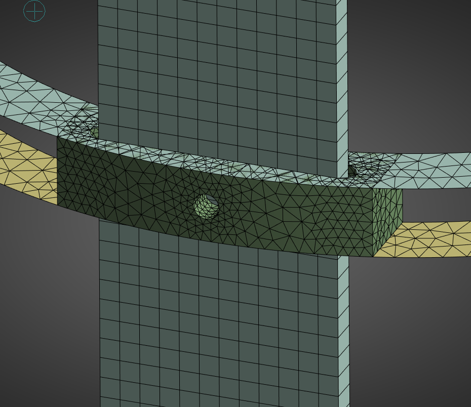
Here is a close up on the spacers and ABR:
Here is a complete view of the mesh quality, where the lowest quality components are the top vertices of the coupler, and some corners in the thrust plate. The overall quality is quite high, specifically on the rods and ABRs.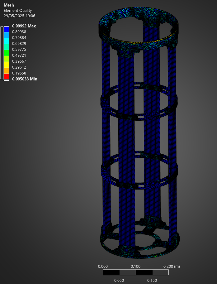
¶ ACP Pre
For the carbon fiber ABRs, we can't obtain their material properties from a software such as Esacomp (as was done for the rods) due to their specific 3D geometry, and the desired fiber orientation.
As such, we have to use the ACP Pre module in Ansys to properly simulate carbon fiber.
In short, ACP Pre allows us to create a carbon fiber lay up, orienting the fibers as desired.
In this secton we will explain exactly how one of the two set ups was done, as the methodology for both is almost identical - this forms the basis of an ACP Tutorial.
First, for an easier time in ACP, you want to work with "shell geometry" to do your lay ups. This means that instead of having a solid body where you expect the carbon fiber to go, you pick a surface on which you will "lay up" carbon fiber - in this case, it is exactly how you would imagine manufacturing the piece.
To do this, we carefully designed our ABRs so that we could delete all the surfaces of the carbon fiber "body," except for the one from which the lay ups would be done.
The removal of the surfaces is done in Ansys Discovery, when adding the geometry to the geometry module.
This is an essential part of ACP Pre to make your life easier.
Careful, if you have a surface which is "part of another surface," using Discovery will remove said surface, and you must do the surface removal on other software. We found it simpler to do this in Fusion360, after trying on Solidworks. In our case the surface on which the engine applies its force is the same surface as the bottom of the coupler, but doesn't cover its entirety - the 3D model has a "line" that separates both surfaces. This line would disappear in Ansys and we could no longer apply the motor's force properly.
Afterwards, in Ansys Mechanical, we created "named selections" for each different carbon fiber lay up we wanted to do. In this case, the ABRs have 4 carbon fiber rings - this means we have 4 named selections. The named selections allow us to have 4 separate lay ups in ACP, instead of one.
Your pre processed ABR should look like the bottom one in this image (the surface is transparent), as opposed to the top one, which is the original 3D model (the rings are solid, and thick).
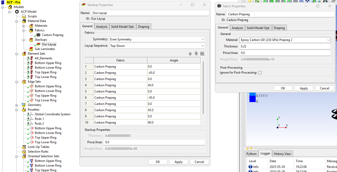
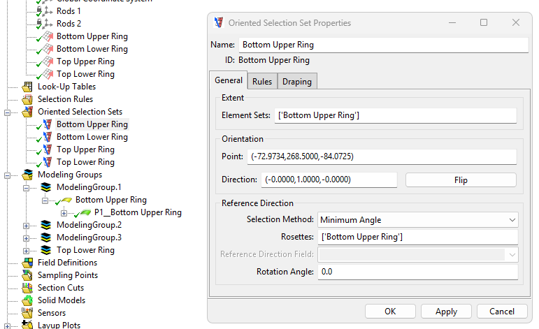
First, in ACP, define the Material Data - Fabrics, and Stackups. Here, choose what material you want to use (previously defined in the Engineering Data tab), its thickness, the amount of layers, and their angles. Careful with the thickness' unit, it can result in very bizarre modes!
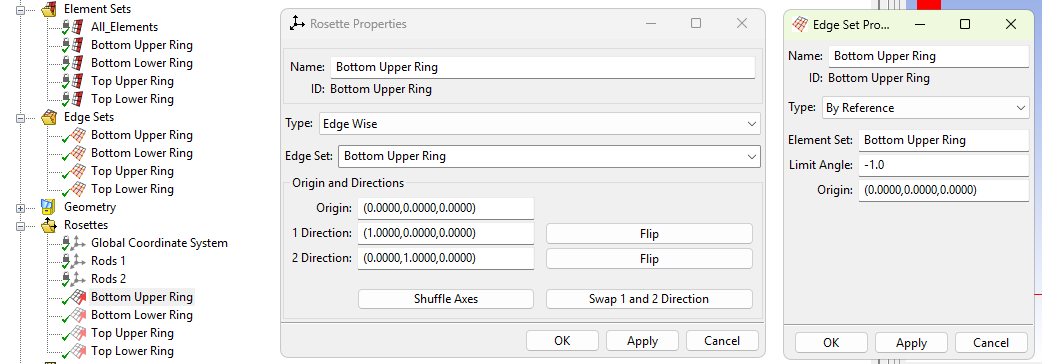
Next, define "Rosettes" which are, essentially, a type of coordinate system that allows ACP to layer the carbon fiber in the way you intend to. There are many options, in our case we used "Edge Sets" which essentially tell ACP to follow the edge, which, for our cylinders, is very practical.
Define the edge sets based on the Element Sets (which are created when you do a Named Selection in Mechanical), and then define rosettes by clicking the model on which you are performing the layup (the one corresponding to your element set), and the corresponding edge set.
 .
.
Create "Oriented Selection Sets." The Oriented Selection brings everything together: choose the element set (model) on which the layup goes, the rosette with which the layup will be oriented, and finally the orientation in which it will be layed up: will you layup "upwards" or "downwards" - in our case, we always orient it in the direction opposing the spacers, as otherwise we would have overlap.
Finally, create Modeling Groups. First, create a modeling group, then, create a "Ply." Choose an Oriented Selection Set, the layup, and, if necessary, a ply angle and a number of layers.
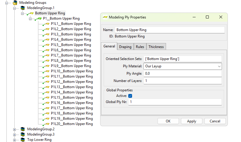
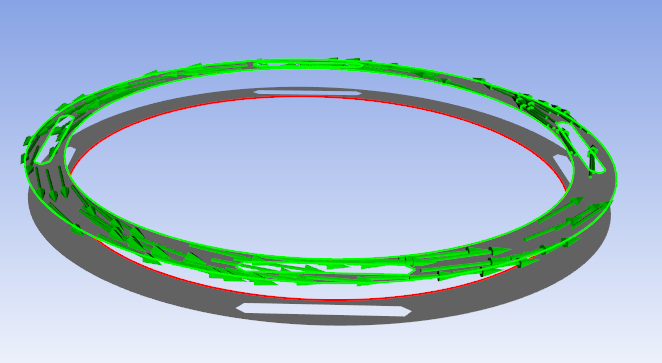
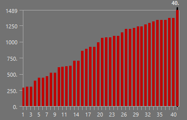
Once this is done, click the lightning logo (or press "Apply") and you will be able to check the orientation of the fibers in the UI, for every single layer.
One of our 0° layers for the SABRs looked like this:
¶ Outputs
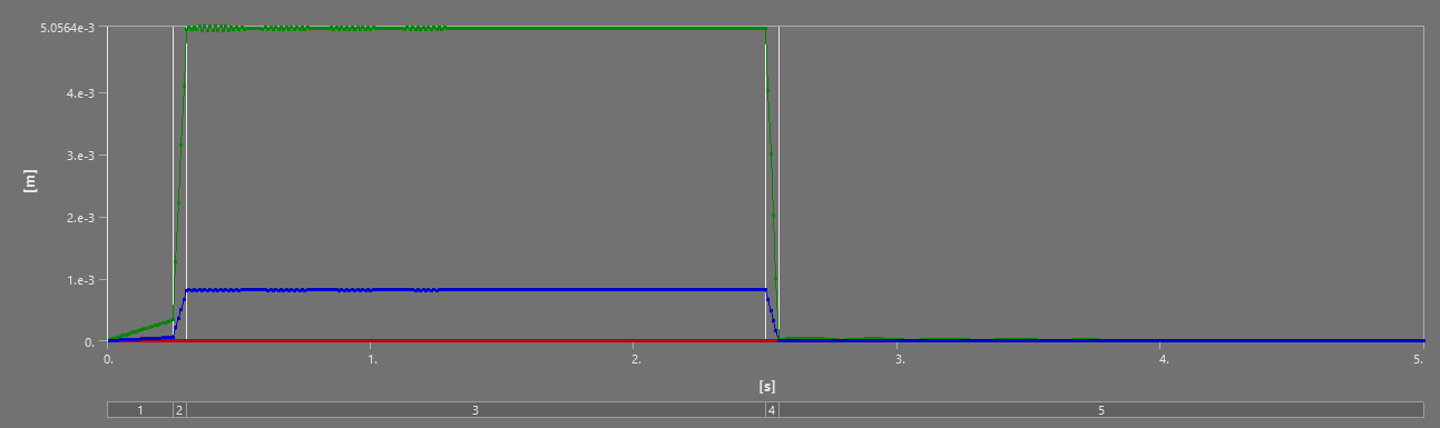
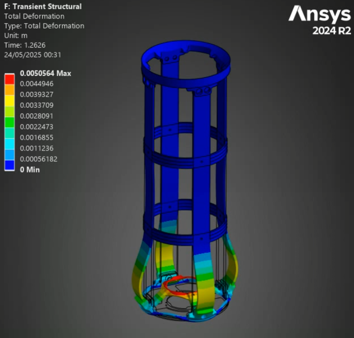
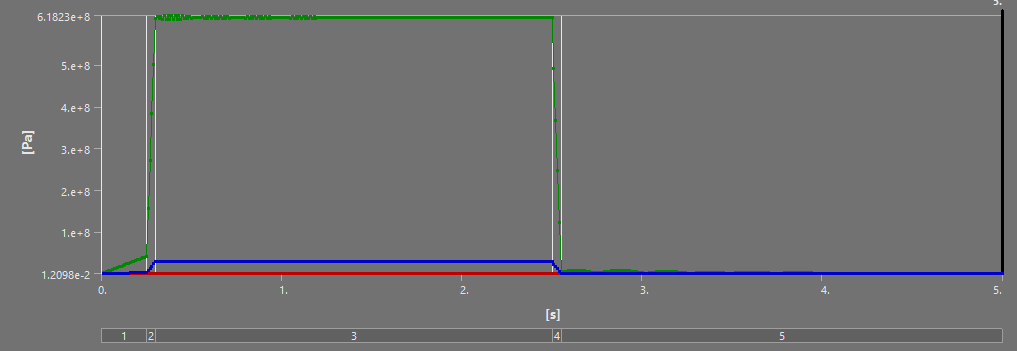
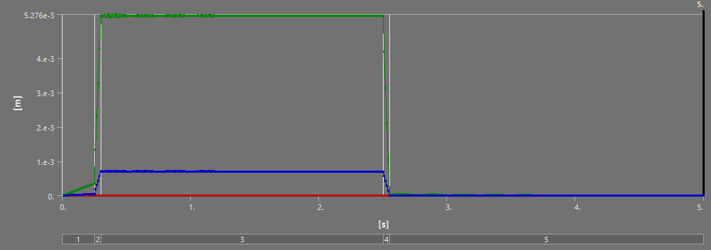
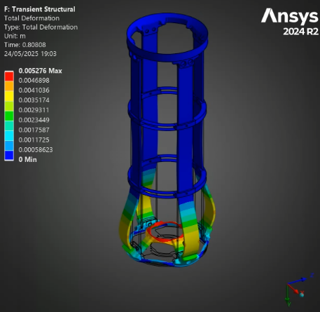
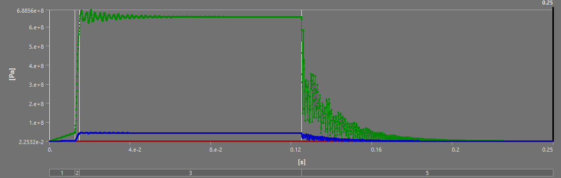
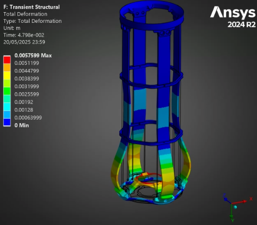
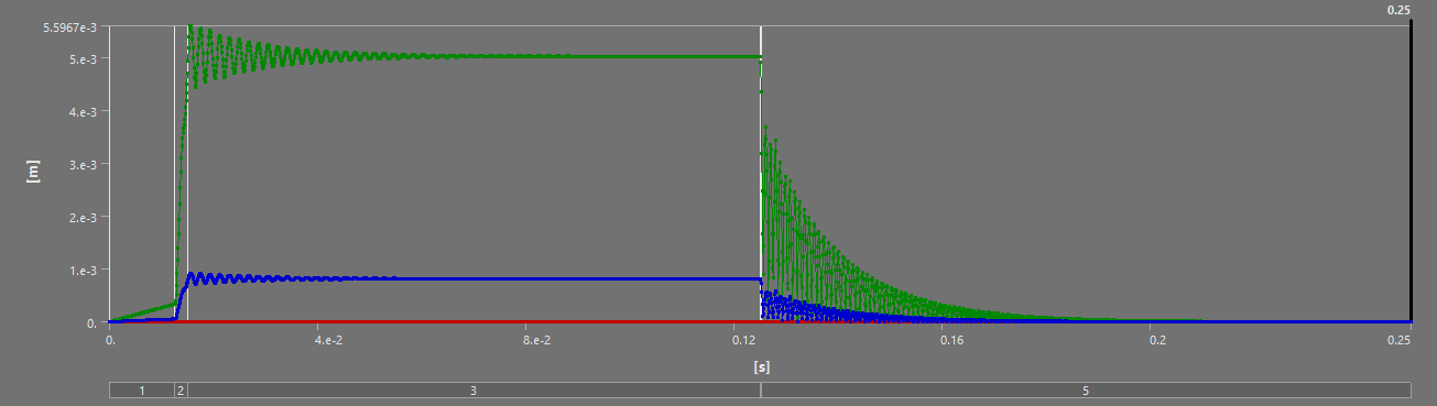
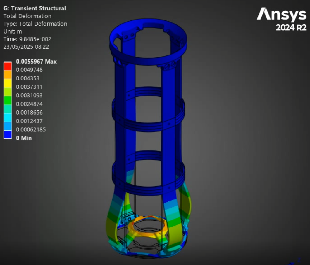
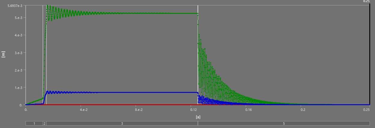
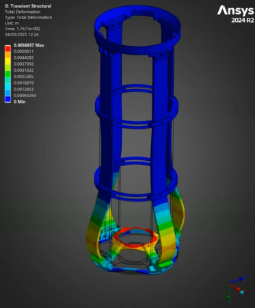
For all of the following simulations, the outputs were videos - as they are transient structural analyses. This report will outline the most interesting states, and show the table of deformation to show the evolution of stress/displacement.
For all of the composite ABRs, the composite failure tool returned extremely high safety factors (1000!) they are not included in these outputs, as, with such a high value that was consistent across both ABR models, and within the model itself, the results are rather uninteresting.
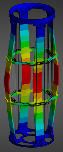
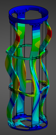
¶ Modes
Given 40 Modes were used, we will simply be showing a table of the modes, and highlighting the first mode, and another, more "fun" mode.
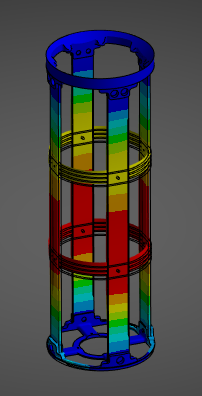
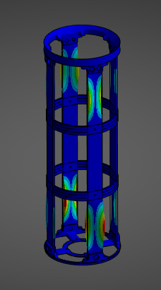
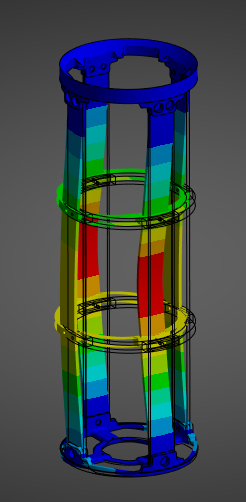
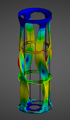
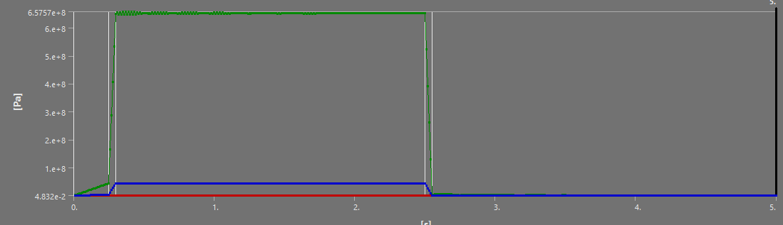
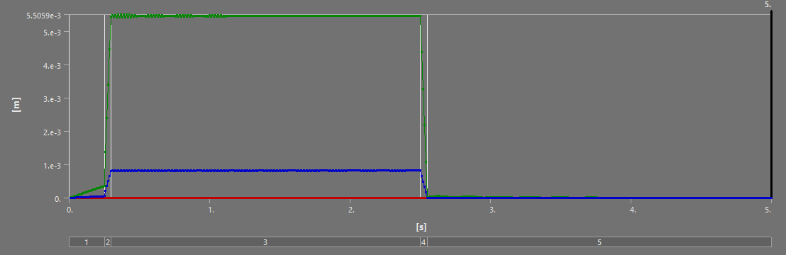
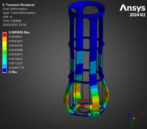
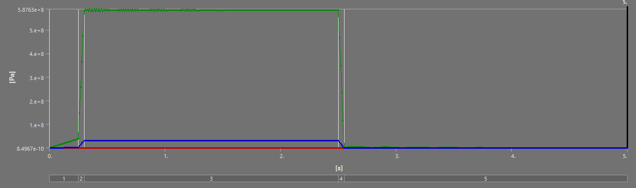
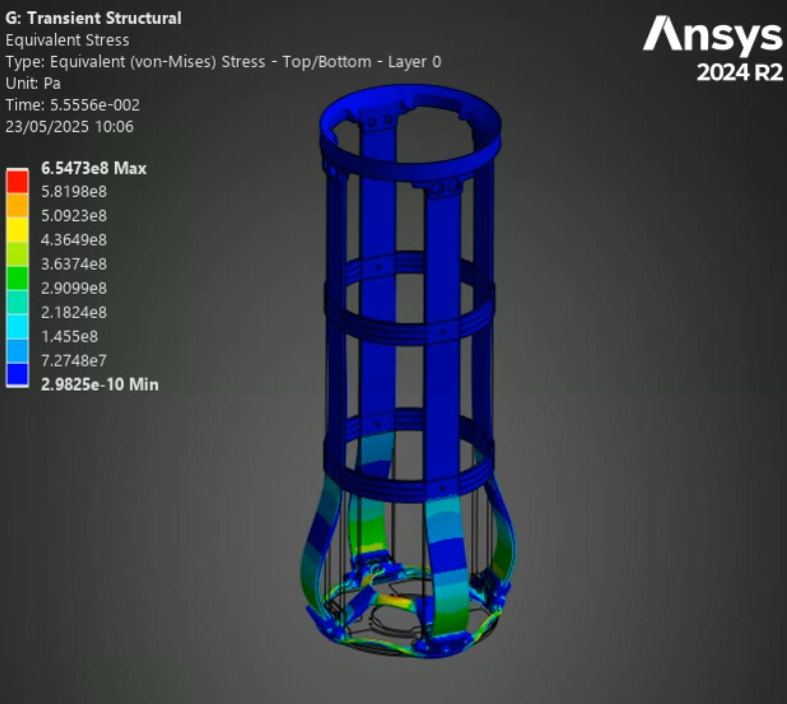
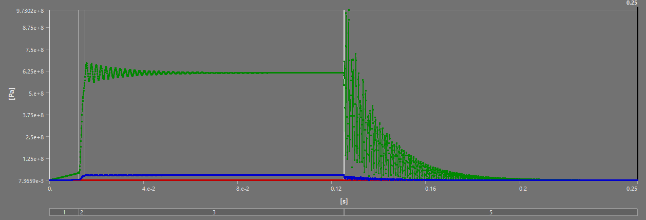
¶ Stress and Displacements

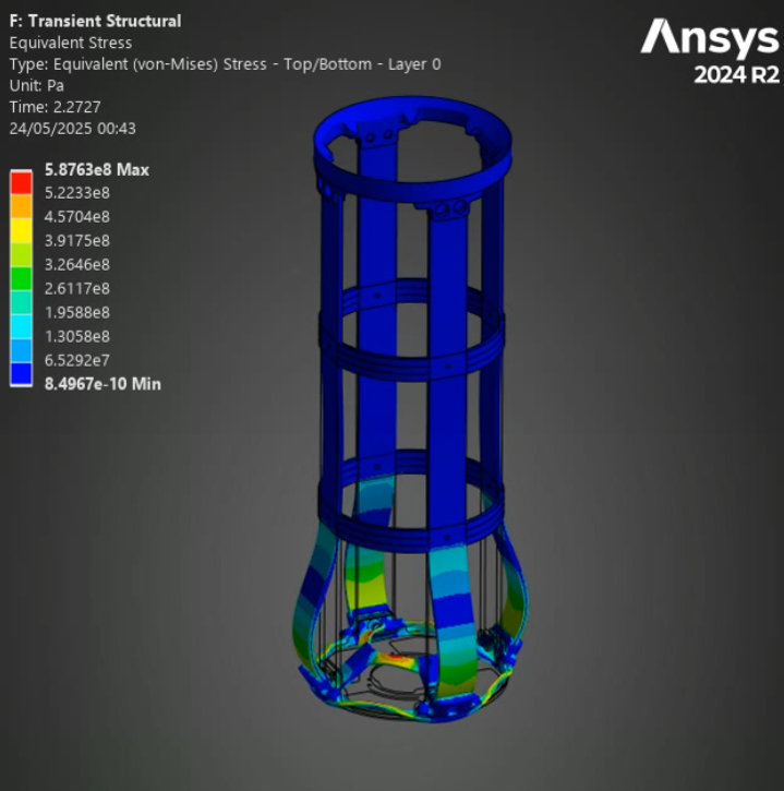
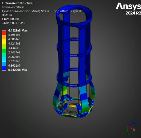
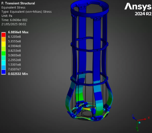
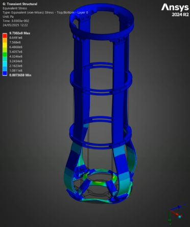
¶ Interpretation
¶ Simulation validity
It's hard to validate this simulation with complete confidence, for two main reasons. One, without a proper mesh convergence analysis, we can never be certain the results have, in fact, converged, and that they are independent of the mesh. Two, the trade offs made due to file size mean we never actually simulated the precise dynamic load experienced by the engine bay, so it is, of course, imperfect.
That being said, the mesh independence tests executed on the same models for the first static simulations and the coherence in results between both short scale and full burn simulations as well as between different ABRs is reassuring as to the validity of these simulations.
In short, while these simulations can definitely be improved, in the current scope, this is sufficient.
¶ Comparisons
¶ Full Burn
| ABR | Mass (g) | Relative Difference | Max Displacement (mm) | Relative Difference | Max Stress (GPa) | Relative Difference |
|---|---|---|---|---|---|---|
| H ABR | 213 | +40% | 5 | -9% | 0.58 | -12% |
| S ABR | 131.6 | -13.4% | 5.2 | -5.5% | 0.62 | -6% |
| Aluminum ABR | 152 | N/A | 5.5 | N/A | 0.66 | N/A |
The full burn validates our past analyses: between the H ABR and S ABR, the SABR has a more optimal performance to mass ratio - it manages to decrease the displacement and stress while lowering the weight. The HABR's performance improvement relative to the aluminum ABR is not sufficient to justify the 40% increase in mass.
¶ Short Scale
| ABR | Mass (g) | Relative Difference | Max Displacement (mm) | Relative Difference | Max Stress (GPa) | Relative Difference |
|---|---|---|---|---|---|---|
| H ABR | 213 | +40% | 5.6 | -3.4% | 0.65 | -1.5% |
| S ABR | 131.6 | -13.4% | 5.7 | -1.7% | 0.97 | +42% |
| Aluminum ABR | 152 | N/A | 5.8 | N/A | 0.68 | N/A |
On the short scale, the SABR's dominance relative to the HABR is once again highlighted - except for the Max Stress. I believe this max stress is due to a force concentration, and doesn't actually reflect reality, as no other such stress has been observed in any of our simulations.
¶ Conculsions
The conclusions of these simulations and their results can be split in two, the educational component, and the actual engineering results.
From an educational point of view, this report sets in motion the possibility of executing not only dynamical analyses in the Rocket Team, but also assembly, with composite, dynamical analyses. Much of the content here could be either condensed into a proper Ansys tutorial, or simply referred to as an applied tutorial. The potential value here for future development is quite high.
In addition, noting that the steady state achieved in both small scale and full burn simulations somewhat validates the approach of "small scaling" the loads and simulating that, to reduce computation time and file size.
From a results point of view, these simulations are a little disappointing, albeit better than the first static ones. The SABR, at least, has equivalent performance to the aluminum ABRs, but with a 15% reduction in weight. The HABR is, once again, quite disappointing.
These results beg the question "aren't composites better than aluminum? how come the aluminum ABRs are that much better?" The answer to this isn't exactly clear, especially given the delta in performance between both our composite ABRs. In our opinion, this indicates a sub optimal use of the carbon's fibers, where some of them are not being used: thus contributing to the mass, but not the performance. A next step in improving these ABRs would be to try to understand which fibers are being used most, and how to maximize this usage. In the SABRs for example, maybe the fibers close to the rods are most used, so the rings could be made to be a little smaller, but thicker.
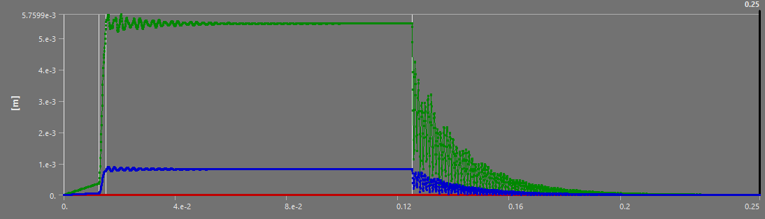
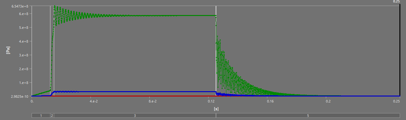
Finally, the stress and displacement results of the thrust plate are very interesting. Although they are not related to our core project, the ability to simulate the oscillations critical pieces like the thrust plate experience during a dynamic load means we can now set requirements that depend on these oscillations. In the small scale simulations, the peak oscillation tended to be about 10% higher than the steady state - with the factors of security currently employed at the rocket team, this would not be critical to the launch vehicle, but having this understanding of oscillations and being able to implement them in our considerations is still highly beneficial. Furthermore, the displacement of the thrust plate could be critical for the plumbing in the engine bay, that, of course, has to move if the engine moves.